Following a trials recruitment is an important task for timing of
analyses and ensuring that a trial will not run for too long (longer
trials are more expensive). accrualPlot provides tools for
easily creating recruitment plots and even for predicting when a trial
will have successfully recruited all participants.
The package is loaded like any other:
library(accrualPlot)
#> Loading required package: lubridate
#>
#> Attaching package: 'lubridate'
#> The following objects are masked from 'package:base':
#>
#>     date, intersect, setdiff, union
The accrual_df
To work with accrualPlot, we need some data,
specifically dates and, optionally, site identifiers. Here’s some data
that we will use in the following examples.
data(accrualdemo)
head(accrualdemo)
#>           date   site
#> 24  2020-07-09 Site 1
#> 87  2020-07-14 Site 1
#> 126 2020-07-14 Site 1
#> 193 2020-07-14 Site 1
#> 139 2020-07-16 Site 1
#> 248 2020-07-19 Site 1accrual_dfs are simply dataframes with the number of
participants on each day participants are recruited (or site) began
recruiting.
Monocentric trials
Monocentric trials obviously have only a single site, so we only need
the x object we just created. We can pass this into the
accrual_create_df function.
df <- accrual_create_df(accrualdemo$date)
print(df, head = TRUE)
#> 250 participants recruited between 2020-07-09 and 2020-10-09
#>         Date Freq Cumulative
#> 1 2020-07-09    0          0
#> 2 2020-07-09    1          1
#> 3 2020-07-14    3          4
#> 4 2020-07-16    1          5
#> 5 2020-07-19    1          6
#> 6 2020-07-20    1          7
In this case, the accrual_df has a single data
frame.
Multicentric trials
For multicentric trials, we should also pass the site identifier to
accrual_create_df in the by argument.
df2 <- accrual_create_df(accrualdemo$date, by = accrualdemo$site)
print(df2, head = TRUE)
#> Site 1:
#> 141 participants recruited between 2020-07-09 and 2020-10-09
#>         Date Freq Cumulative
#> 1 2020-07-09    0          0
#> 2 2020-07-09    1          1
#> 3 2020-07-14    3          4
#> 4 2020-07-16    1          5
#> 5 2020-07-19    1          6
#> 6 2020-07-21    1          7
#>
#> Site 2:
#> 88 participants recruited between 2020-07-20 and 2020-10-09
#>         Date Freq Cumulative
#> 1 2020-07-20    0          0
#> 2 2020-07-20    1          1
#> 3 2020-07-21    1          2
#> 4 2020-07-22    1          3
#> 5 2020-07-23    1          4
#> 6 2020-07-26    1          5
#>
#> Site 3:
#> 21 participants recruited between 2020-09-04 and 2020-10-09
#>         Date Freq Cumulative
#> 1 2020-09-04    0          0
#> 2 2020-09-04    1          1
#> 3 2020-09-05    1          2
#> 4 2020-09-07    2          4
#> 5 2020-09-12    1          5
#> 6 2020-09-13    1          6
#>
#> Overall:
#> 250 participants recruited between 2020-07-09 and 2020-10-09
#>         Date Freq Cumulative
#> 1 2020-07-09    0          0
#> 2 2020-07-09    1          1
#> 3 2020-07-14    3          4
#> 4 2020-07-16    1          5
#> 5 2020-07-19    1          6
#> 6 2020-07-20    1          7
In this case, the accrual_df is a list of dataframes,
one for each site and an overall.
Start and end dates
By default, the start and end dates are defined based on the dates
that you pass to accrual_create_df. You can override these
via the start_date and current_date arguments.
This is useful for when you have particularly slow recruiting trials
(such as those with particularly strict inclusion criteria). For
example, our fictitious example trial might have started recruiting on
the 1st November. By adding this information, we modify other output
df3 <- accrual_create_df(accrualdemo$date, start_date = as.Date("2020-07-08"))For multicentric trials where different sites started recruiting at
different times, we can pass a vector to start_date
start_date<-as.Date(c("2020-07-09","2020-07-09","2020-08-01"))
names(start_date)<-c("Site 1","Site 2","Site 3")
df4 <- accrual_create_df(accrualdemo$date, by = accrualdemo$site, start_date = start_date)
Accrual plots
accrualPlot has three flavours of plots:
* Cumulative
* Absolute
* Prediction
and supplies both base graphics as well as ggplot2
graphics implementations (allowing easier modification).
Cumulative plots
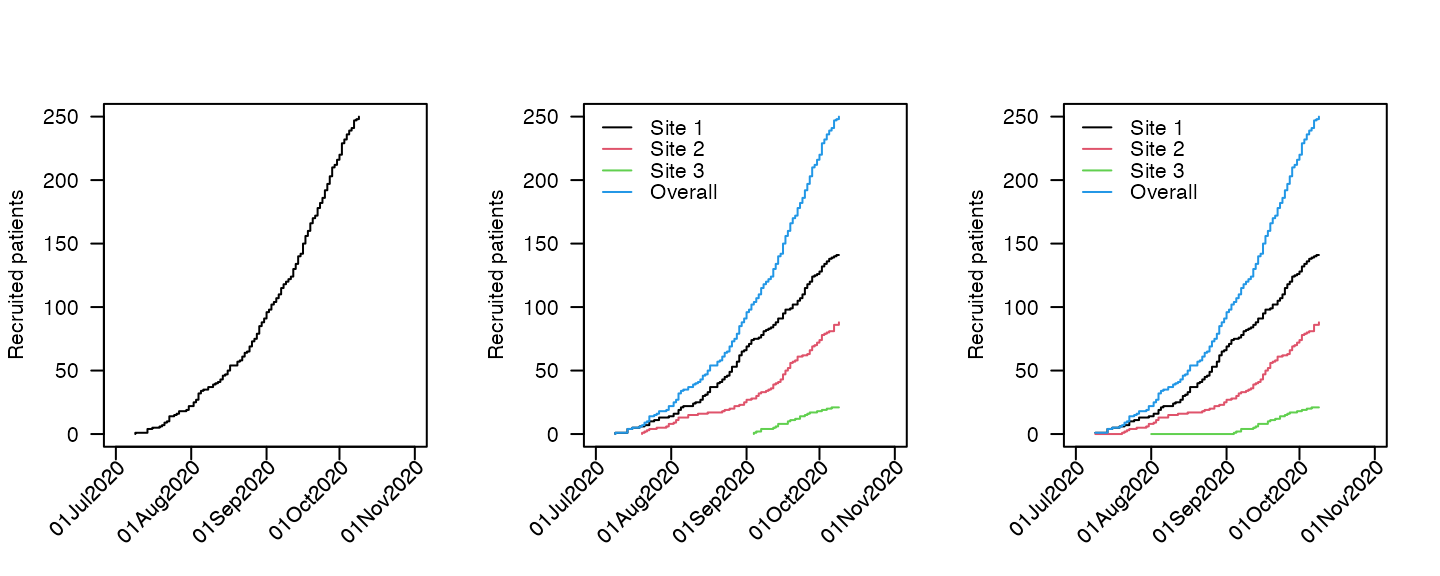
Cumulative plots show a standard step function of the number of
participants recruited up to a given point in time. The plots are
produced via the plot method (which is a wrapper for the
internal function accrual_plot_cum)
For ggplot2 graphics, use the engine option:
library(patchwork)
library(ggplot2)
p1 <- plot(df, engine = "ggplot")
p2 <- plot(df2, engine = "ggplot") +
   theme(axis.text.x = element_text(angle = 45, vjust = 1, hjust=1),
         axis.title.x = element_blank())
p3 <- plot(df4, engine = "ggplot") +
  labs(col = "Site") +
  theme_classic() +
  theme(legend.position = c(.35,.9),
     legend.key.height = unit(2, "mm"),
         legend.text=element_text(size=8),
         legend.title=element_blank(),
     axis.text.x = element_text(angle = 45, vjust = 1, hjust=1),
         axis.title.x = element_blank())
#> Warning: A numeric `legend.position` argument in `theme()` was deprecated in ggplot2
#> 3.5.0.
#> ℹ Please use the `legend.position.inside` argument of `theme()` instead.
#> This warning is displayed once every 8 hours.
#> Call `lifecycle::last_lifecycle_warnings()` to see where this warning was
#> generated.
p1 + p2 + p3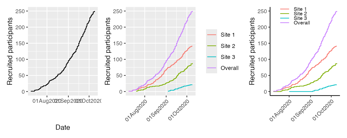
Absolute recruitment
Recruitment plots per unit time can be obtained via the
absolute method (specify which = "absolute" to
plot)
par(mfrow = c(1, 3))
plot(df, which = "abs", unit = "week")
plot(df2, which = "abs", unit = "week", legend.list=list(x="topleft"), xlabsel=seq(1,20,by=2))
plot(df4, which = "abs", unit = "month",legend.list=list(x="topleft"))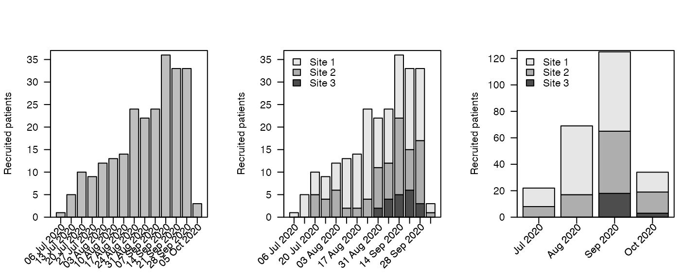
Options for unit are year,
month, week and day.
Where multiple sites exist, the different sites are indicated by different colours on the stacked bars.
p1 <- plot(df, which = "abs", unit = "week", engine = "ggplot")
p2 <- plot(df2, which = "abs", unit = "week", engine = "ggplot") +
    theme(axis.text.x = element_text(angle = 45, vjust = 1, hjust=1),
         axis.title.x = element_blank())
p3 <- plot(df4, which = "abs", unit = "month", engine = "ggplot") +
  labs(fill = "Site") +
  theme_classic() +
  theme(legend.position = c(0.01,0.9),
     legend.justification = "left",
     legend.key.height = unit(2, "mm"),
     legend.key.width = unit(2, "mm"),
         legend.title=element_blank(),
     axis.text.x = element_text(angle = 45, vjust = 1, hjust = 1),
         axis.title.x = element_blank())
p1 + p2 + p3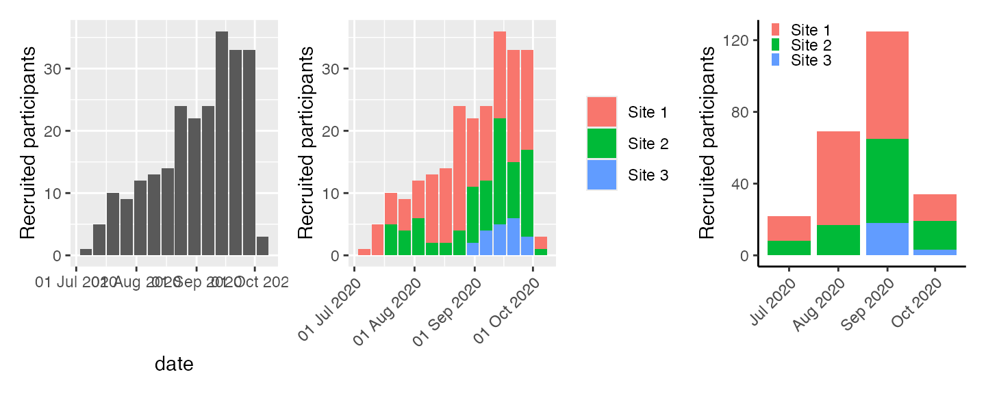
It might be desirable to have panels for each site. This is easy to
do with the ggplot implementation. The variable to use in
this case is site, which is constructed in the appropriate
plot function.
plot(df2, which = "abs", unit = "week", engine = "ggplot") + facet_wrap(~site)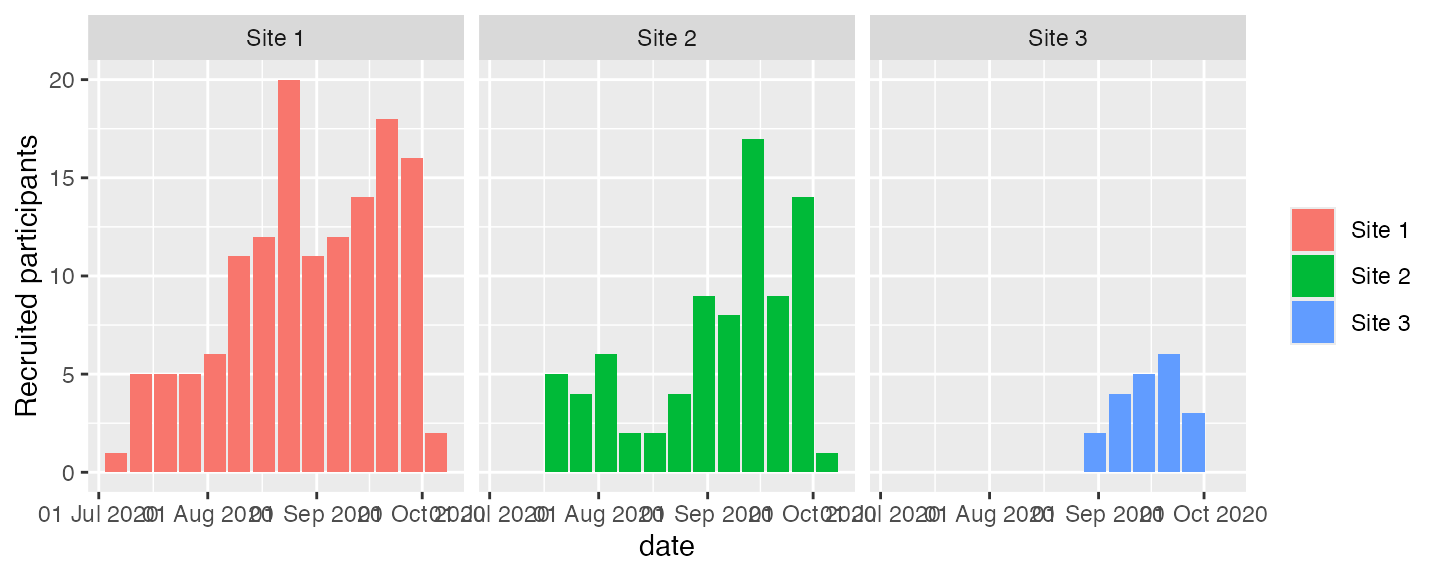
Date at which a target sample size is reached
In order predict the time point at which a certain number of
participants has been recruited (for estimating when a study will be
complete). If we want to recruit a total of 300 participants, we can put
that in the target option.
par(mfrow = c(1, 3))
plot(df, which = "predict", target = 300, cex_prediction=0.9)
plot(df2, which = "predict", target = 300, cex_prediction=0.9)
plot(df4, which = "predict", target = 300, cex_prediction=0.9,  center_legend="strip")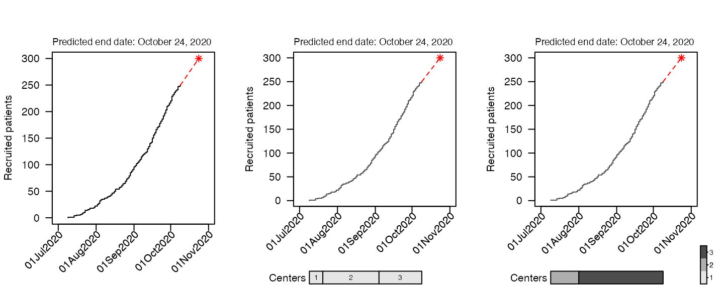
We can also include site-specific targets:
plot(df4, which = "predict", target=c("Site 1"=160,"Site 2"=100,"Site 3"=40,"Overall"=300),
     show_center=FALSE)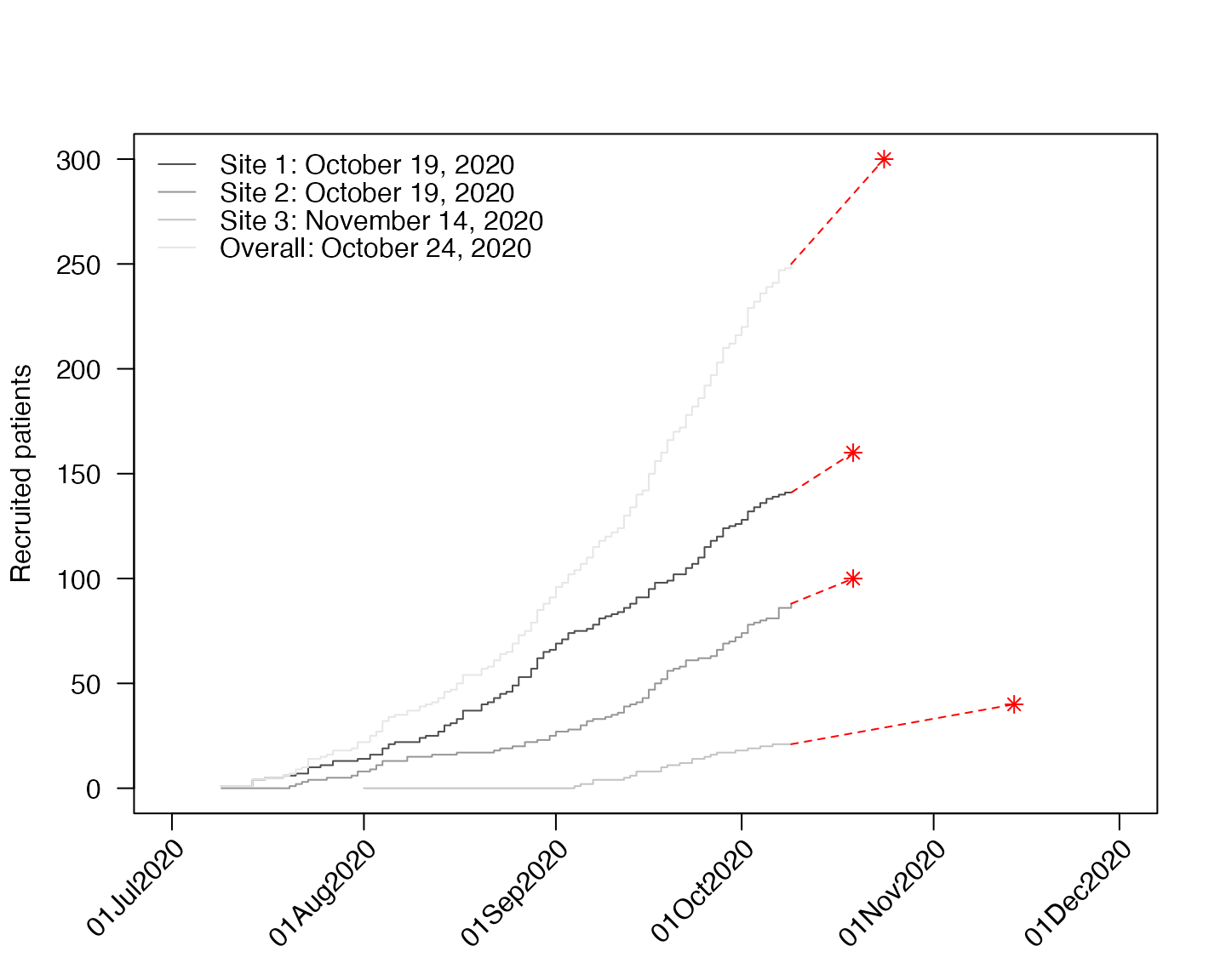
Or with ggplot2.
p1 <- plot(df, which = "predict", target = 300, engine = "ggplot2") +
  theme(plot.title.position = "plot")
p2 <- plot(df2, which = "predict", target=c("Site 1"=160,"Site 2"=100,"Site 3"=40,"Overall"=300),
  engine = "ggplot2") +
  labs(col = NULL) +
  theme_classic() +
  theme(legend.position = c(.025,.9),
        legend.justification = "left",
        legend.key.height = unit(2, "mm"),
        legend.key.width = unit(2, "mm"),
        legend.background = element_rect(fill = NA),
        axis.text.x = element_text(angle = 45, vjust = 1, hjust = 1),
        axis.title.x = element_blank())
p1 + p2
#> Warning in geom_point(aes(x = edate, y = targetm), col = col.pred, pch = pch.pred): All aesthetics have length 1, but the data has 79 rows.
#> ℹ Please consider using `annotate()` or provide this layer with data containing
#>   a single row.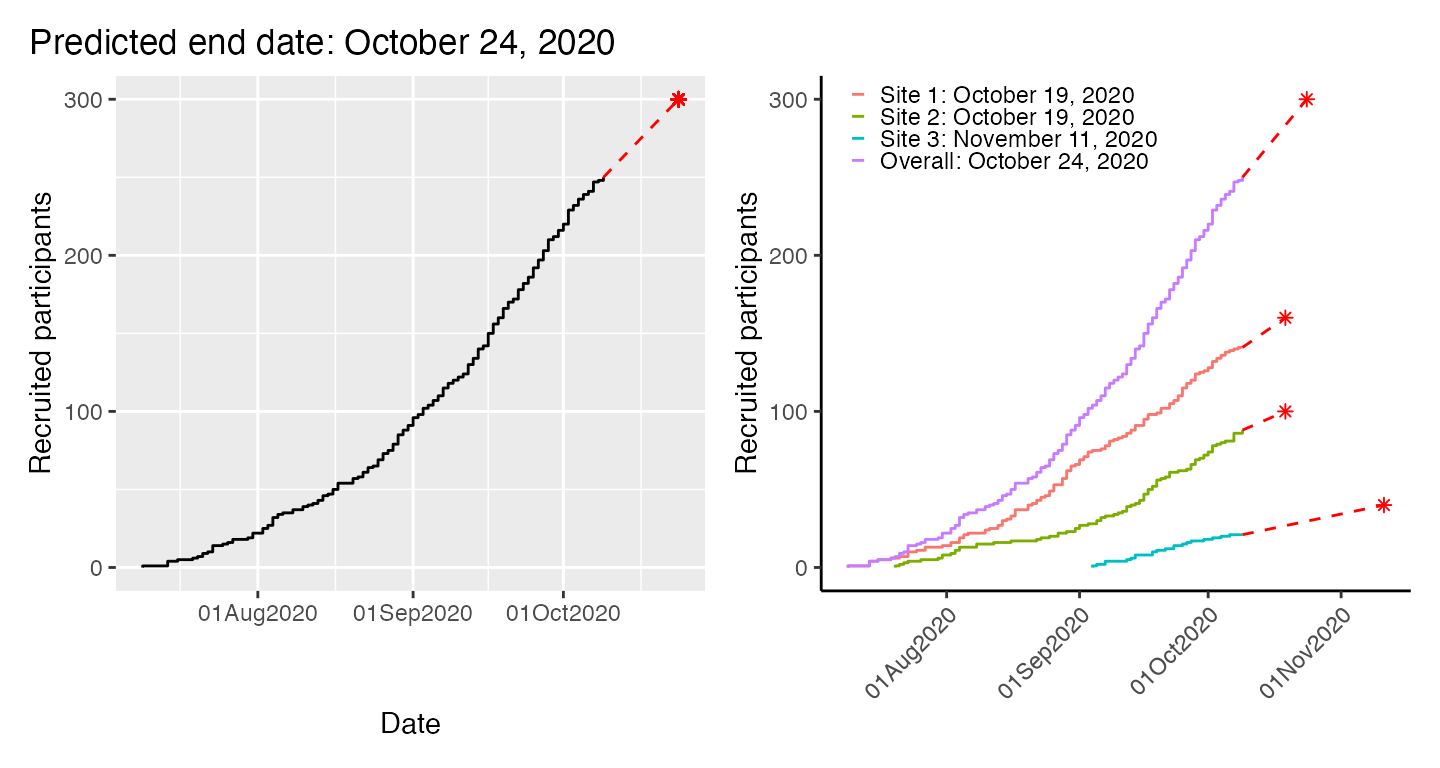
In the second ggplot2 example above, we specify
different targets for each site, plus a study-level target. The syntax
is the same for base graphics.
It’s not strictly necessary to use plot for any of the
above figures. plot is a wrapper which selects one of 6
underlying functions depending on the value of the which
and engine arguments. The underlying functions for base
graphics are accrual_plot_cum for cumulative plots,
accrual_plot_abs for absolute values, and
accrual_plot_predict for the prediction plots. The
ggplot equivalents just prepend those names with
gg_, i.e. gg_accrual_plot_cum,
gg_accrual_plot_abs and
gg_accrual_plot_predict. For more clarity, it might be
desirable to use those instead, e.g.
gg_accrual_plot_predict(df2, target=c("Site 1"=160,"Site 2"=100,"Site 3"=40,"Overall"=300))Sample size at a specific time point
It is also possible to predict the expected sample size at a specific
time point. If we want to know how many patients will be recruited at
the end of the year, we can put the date in the target
option.
par(mfrow = c(1, 2))
plot(df4, which = "predict", target = as.Date("2020-12-31"), cex_prediction=0.9,  center_legend="strip")
target<-rep(as.Date("2020-12-31"),4)
names(target)<-c("Site 1","Site 2","Site 3","Overall")
plot(df4, which = "predict", target=target,show_center=FALSE)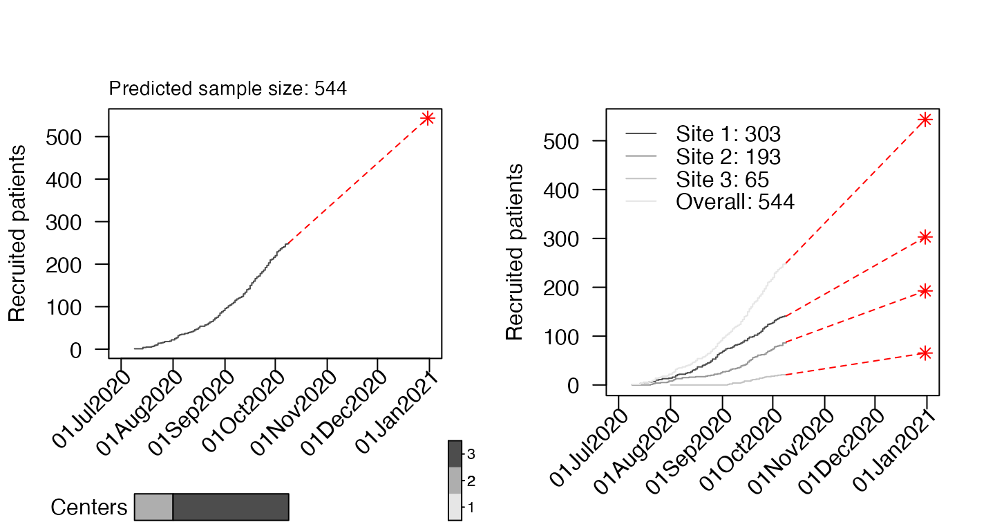
In the second example we get site-specific predicions using a target vector (with the same date for all sites). Please note that the site-specific estimates do not necessarily sum up to the overall because they are derived from separate models.
Recruitment tables
Tables of recruitment can also be generated using
accrualPlot, via the summary method. As with
absolute recruitment above, a unit of time can be specified.
# accrual_table(df)
summary(df, unit = "day")
#>             start_date          time                    n
#> 1 First participant in Days accruing Participants accrued
#> 2            09Jul2020            92                  250
#>                     rate
#> 1 Accrual rate (per day)
#> 2                   2.72
summary(df2, unit = "day")
#>      name           start_date          time                    n
#> 1  Center First participant in Days accruing Participants accrued
#> 2  Site 1            09Jul2020            92                  141
#> 3  Site 2            20Jul2020            81                   88
#> 4  Site 3            04Sep2020            35                   21
#> 5 Overall            09Jul2020            92                  250
#>                     rate
#> 1 Accrual rate (per day)
#> 2                   1.53
#> 3                   1.09
#> 4                   0.60
#> 5                   2.72
summary(df3, unit = "day")
#>             start_date          time                    n
#> 1 First participant in Days accruing Participants accrued
#> 2            08Jul2020            93                  250
#>                     rate
#> 1 Accrual rate (per day)
#> 2                   2.69
summary(df3, unit = "day", header = FALSE)
#>   start_date time   n rate
#> 1  08Jul2020   93 250 2.69